1  Basics

Keywords

statistics, modelling, introduction, course, data analysis, R

1.1 Embarking

Exercise 1.1 (Hello stats) Present yourself to the group along the lines of the following three tags:

1. Your primary scientific interest
2. Your expectations to this course
3. Your background in statistics and R

If you want, feel free to add a fun fact. \(\square\)

1.2 Goals in statistics

1.2.1 Taxonmy of goals

Many stories to be told. Here’s one, on the goals pursued in statistics (and related fields), see Figure 1.1.

flowchart LR
  A{Goals} --> B(describe)
  A --> C(predict)
  A --> D(explain)
  B --> E(distribution)
  B --> F(assocation)
  B --> G(extrapolation)
  C --> H(point estimate)
  C --> I(interval)
  D --> J(causal inference)
  D --> K(population)
  D --> L(latent construct)

Figure 1.1: A taxonomy of statistical goals

Note

Note that “goals” do not exist in the world. We make them up in our heads. Hence, they have no ontological existence, they are epistemological beasts. This entails that we are free to devise goals as we wish, provided we can convince ourselves and other souls of the utility of our creativity.

Hernán et al. (2019) distinguish:

• Description: “How can women aged 60–80 years with stroke history be partitioned in classes defined by their characteristics?”

• Prediction: “What is the probability of having a stroke next year for women with certain characteristics?”

• Causal inference: “Will starting a statin reduce, on average, the risk of stroke in women with certain characteristics?”

1.2.2 Lab: Your goals

Match your (most pressing) research goal to the nomenclature for scientific goals as shown in Figure 1.1. Explain your reasoning.

Next, put three research themes or studies you particularly like to this nomenclature and explain your reasoning.

1.3 Data analysis as a step-by-step recipe

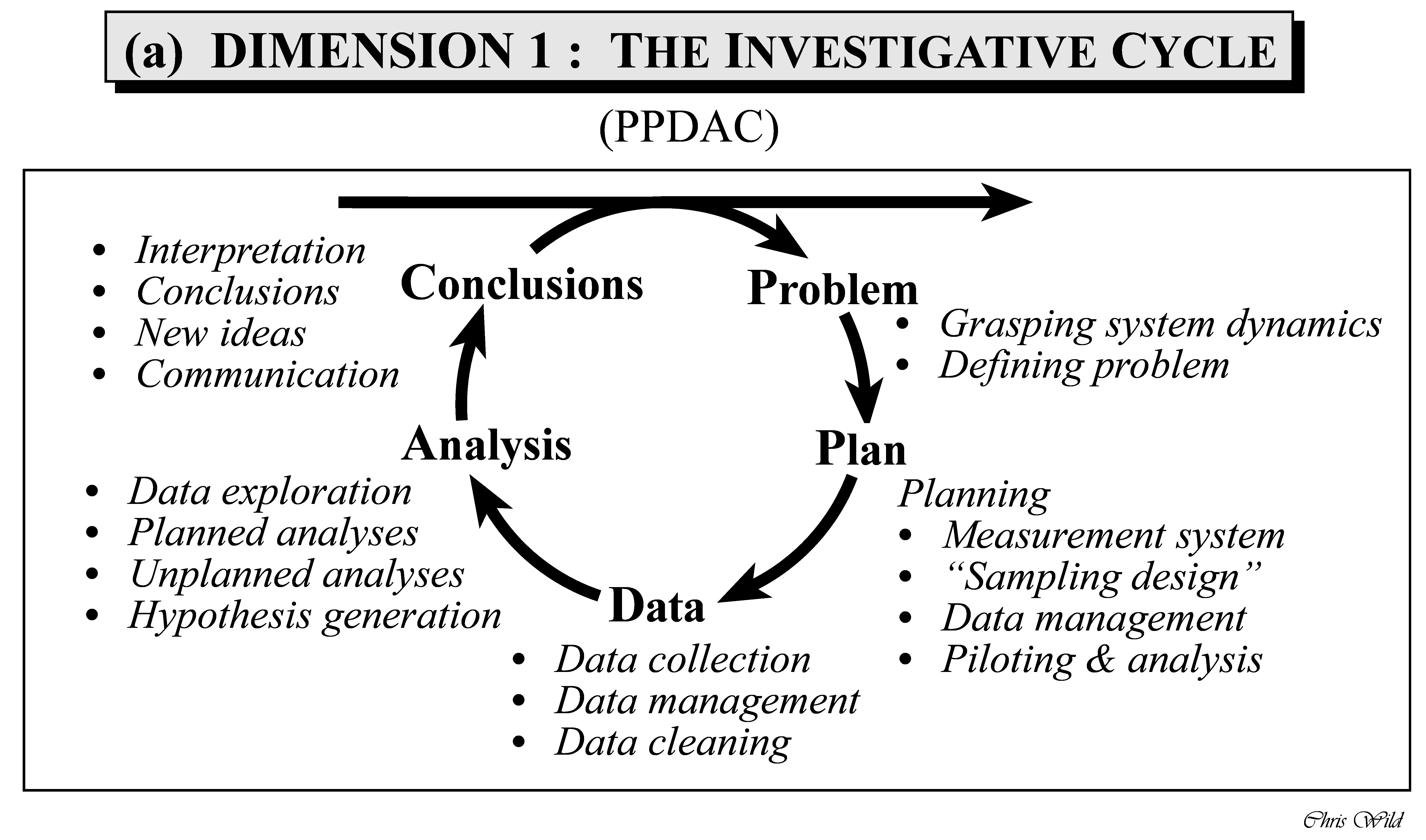
1.3.1 PPDAC

The PPDAC Model is a methodological framework (aka a model) for applying the scientific method to any analytical or research question, or at least it is applicable to quite a few (MacKay & Oldford, 2000). It is not meant to be a rigid sequence, but rather a cycle that may turn a number of rounds like a spiral. Statistician Chris Wild puts the PPDAC cycle in the following figure, see Figure Figure 1.2. In this short essay, he summaries his ideas on how to use the PPDAC as a tool for data analysis in problem solving.

Figure 1.2: PPDAC cycle. Image source: Chris Wild

Wickham and Grolemund (see Figure Figure 2.1 in Section 2.3) provide a suggestion of the parts of the statistical analyses, that is the “Analysis” step in the PPDAC.

1.3.2 Seven steps of data analysis

Data analysis can be conceived as the idea of executing a number of subsequent steps, similar to a cooking receipe.

Figure 1.3 proposes “the seven steps of data analysis”.¹

Actually, there are nine steps in Figure 1.3. As two of which are not directly concerned with data analysis, you may not disagree too strongly with the notion of seven steps.

flowchart LR
  subgraph F[Framework]
    direction LR
    subgraph P[Preparation]
      direction TB
      I[Importing] --> T[Transforming]
    end
    subgraph B[One variable models]
      direction TB
      B1[Point Models] --> V[Visualization]
      V --> U[Variability 1]
    end
    subgraph L[Multiple variables Models]
      direction TB
      L1[(Linear Models)] --> L2[Variability 2]
    end  
    subgraph R[Reporting]
      direction TB
      R1[Writing up] --> R2[Hoping for the best]
    end
  end

  P --> B
  B --> L
  L --> R

Figure 1.3: The ‘seven steps of data analysis’

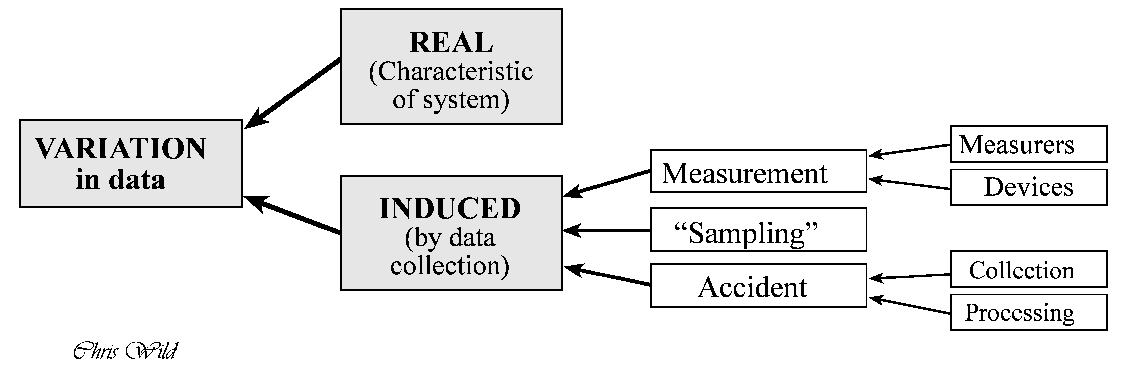
1.4 Variability as the focus of data analysis

Wild & Pfannkuch (1999) further note that variation is one of the essential characteristics of data. They discern to types of variation however, see Figure Figure 1.4.

Figure 1.4: Two types of variartion. Image source: Chris Wild

Wild & Pfannkuch (1999) give a more systematic overview on how a quantitative research question - applied or basic - can be tackled and conceived. For example, in their paper the authors enumarate some dispositions that researcher should embrace in order to fruitfully engage in empirical research:

• Scepticism
• Imagination
• Curiosity
• Opennness
• A propensity to seek deeper menaing
• Being logical
• Engagement
• Perseverance

1.5 Getting started

1.5.1 R Basics

Check out the course Statistics1, chapter on importing data for an accessible introduction to getting started with R and RStudio.

Please also note that R and RStudio should be installed before starting (this course).

In addition, your R packages should be updtodate, according to Arnold Schwarzenegger (s. Figure 1.5).

Figure 1.5: Keep your R packages uptodate, or risk being an outdated model, Arnie says

1.5.2 Help me, I’m lost

Check-out this introductory statistics course.

Pro-Tipp: Use the translation tool of your browser to translate into your favorite language.

1.5.3 Initial quiz

To get an idea whether you have digested some R basics, consider this quiz.

1.6 Blitz start with data

Check out chapter 3 in Statistics1 on how to import data into RStudio and for some basic concepts about “tidy data”.

Spoiler: There’s a button in RStudio in the “Environment” Pane saying “Import Dataset”. Just click it, and things should work out.

Note

I strongly advice working with Projects in RStudio, as it makes working with file paths a lot easier.

We’ll work predominantly with the following data sets.

1.6.1 Motor Trends Cars

To blitz start with data, type the following in R:

data(mtcars)

And the data set mtcars will be available.

To get help for the data set, type help(mtcars)

1.6.2 Penguins

Allez, penguins! Image Credit: Allison Horst, CCO

A bit more advanced, but it’s a nice data set, try the Palmer Penguins data set:

d <- read.csv("https://vincentarelbundock.github.io/Rdatasets/csv/palmerpenguins/penguins.csv")

head(d)  # see the first few rows, the "head" of the table

rownames	species	island	bill_length_mm	bill_depth_mm	flipper_length_mm	body_mass_g	sex	year
1	Adelie	Torgersen	39.1	18.7	181	3750	male	2007
2	Adelie	Torgersen	39.5	17.4	186	3800	female	2007
3	Adelie	Torgersen	40.3	18.0	195	3250	female	2007
4	Adelie	Torgersen	NA	NA	NA	NA		2007
5	Adelie	Torgersen	36.7	19.3	193	3450	female	2007
6	Adelie	Torgersen	39.3	20.6	190	3650	male	2007

Here’s some documentation (code book) for this data set.

1.6.3 Mariokart

Hello Mario, see Figure 1.6!

The data set Mariokart is available via the R package {openintro}.

data("mariokart", package = "openintro") # Paket muss installiert sein

Alternatively, you can download and import it from the Web, see Listing 1.1.

Listing 1.1: Mariokart-Datensatz importieren (mit read.csv)

mariokart <- read.csv(  "https://vincentarelbundock.github.io/Rdatasets/csv/openintro/mariokart.csv")

Figure 1.6: Hello, Mario

Hernán, M. A., Hsu, J., & Healy, B. (2019). A Second Chance to Get Causal Inference Right: A Classification of Data Science Tasks. Chance, 32(1), 42–49. https://doi.org/10.1080/09332480.2019.1579578

MacKay, R. J., & Oldford, R. W. (2000). Scientific Method, Statistical Method and the Speed of Light. Statistical Science, 15(3), 254–278. https://doi.org/10.1214/ss/1009212817

Wild, C. J., & Pfannkuch, M. (1999). Statistical thinking in empirical enquiry. International Statistical Review, 67(3), 223–248.

---

1. Keep in mind that this is magical language. However, it sounds nice and it’s not bad unless you forgot that this is only of multiple ideas of how to do data analysis.