4 Modelling and regression

4.1 Setup

The following R packages are needed for this chapter.

library(easystats)
library(tidyverse)
library(rstanarm)  # optional!
library(ggpubr)  # data visualization

4.2 What’s modelling?

Read this great introduction by modelling by Russel Poldrack. Actually, the whole book is nice Poldrack (2022).

An epitome of modelling is this, let’s call it the fundamental modelling equation, a bit grandiose but at the point, see Equation 4.1.

The data can be separated in the model’s prediction and the rest (the “error”), i.e., what’s unaccounted for by the model.

\[ \text{data} = \text{model} + \text{error} \tag{4.1}\]

A more visual account of our basic modelling equation is depicted in Figure 4.1.

flowchart LR
  X --> Y
  error --> Y

Figure 4.1: A more visual account of our basic modelling equation

4.2.1 Regression as the umbrella tool for modelling

Source: Image Flip

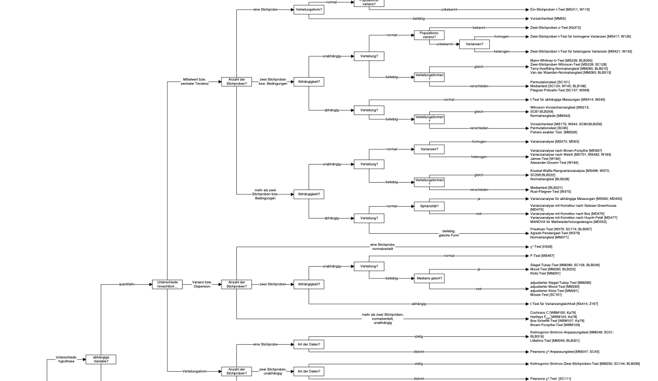
Alternatively, venture into the forest of statistical tests as outlined e.g. here, at Uni Muenster. Proceed at your own peril.

You may want to ponder on this image of a decision tree of which test to choose, see Figure Figure 4.2.

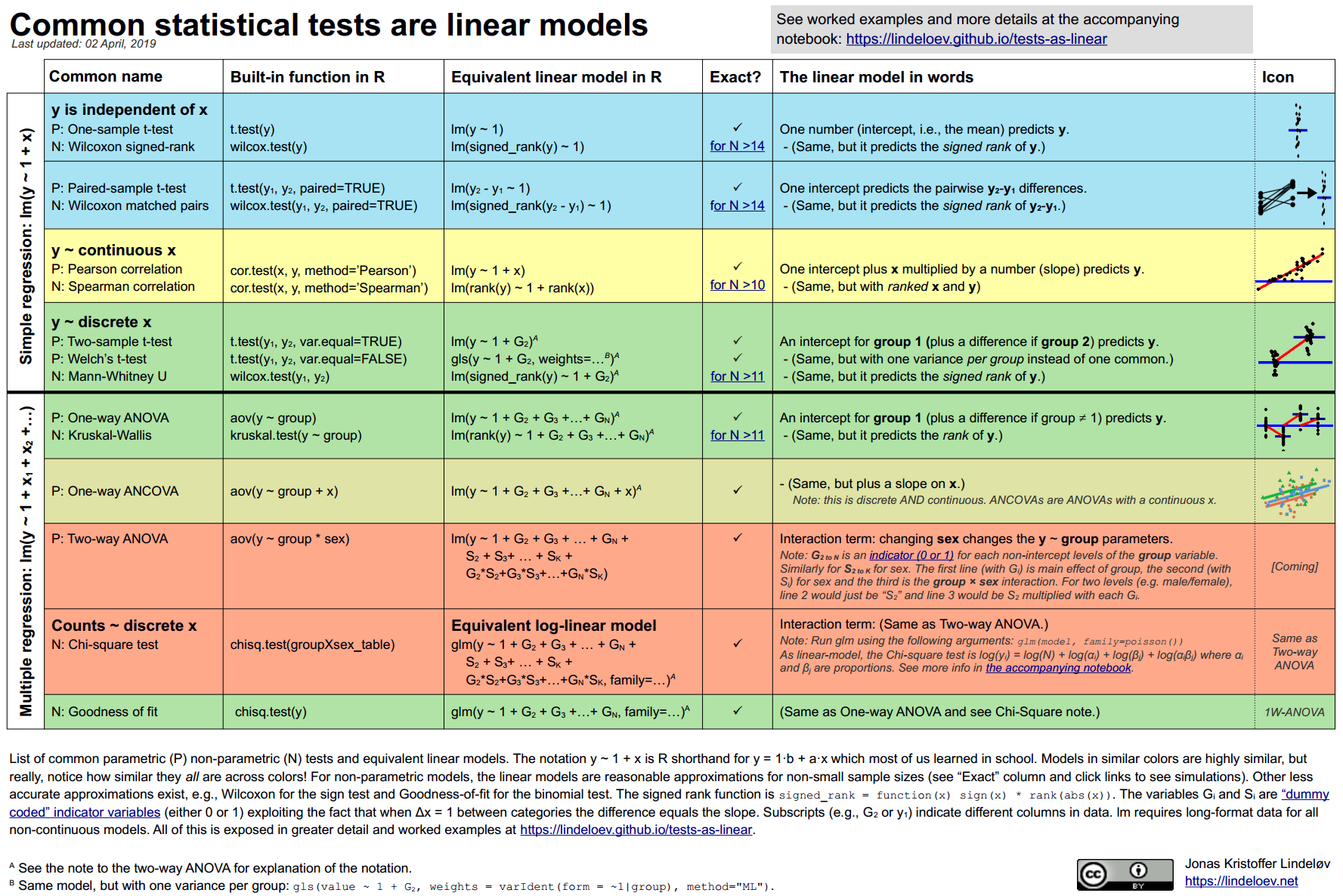
4.2.2 Common statistical tests are linear models

As Jonas Kristoffer Lindeløv tells us, we can formulate most statistical tests as a linear model, ie., a regression.

Common statistical tests as linear models

4.2.3 How to find the regression line

In the simplest case, regression analyses can be interpreted geometrically as a line in a 2D coordinate system, see Figure Figure 4.3.

Source: Orzetoo, CC-SA, Wikimedia

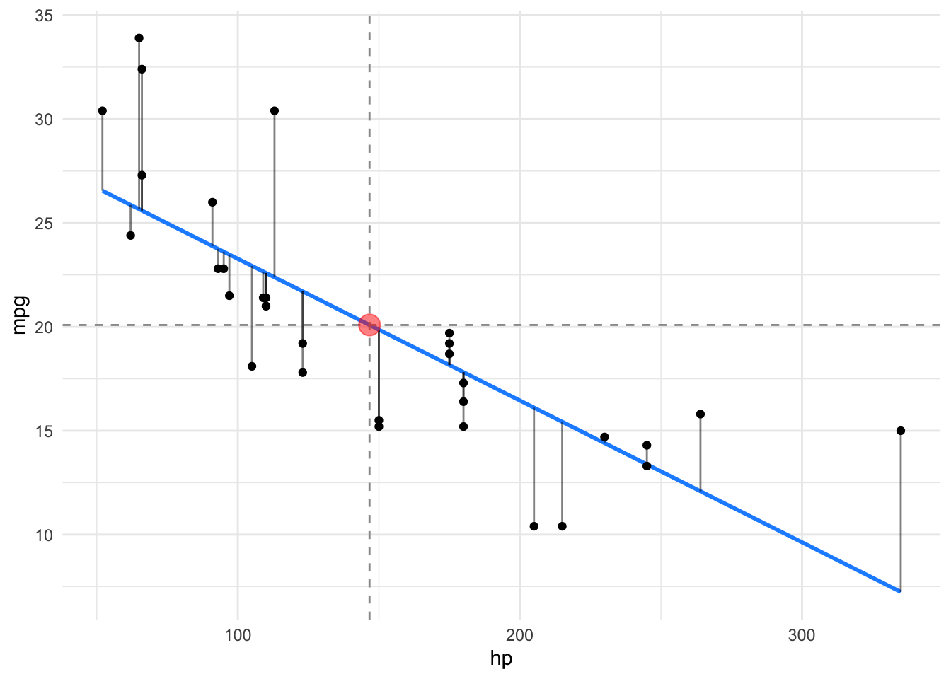
Put simple, we are looking for the line which is in the “middle of the points”. More precisely, we place the line such that the squared distances from the line to the points is minimal, see Figre Figure 4.3.

Consider Figure Figure 4.4, from this source by Roback & Legler (2021). It visualizes not only the notorious regression line, but also sheds light on regression assumptions, particularly on the error distribution.

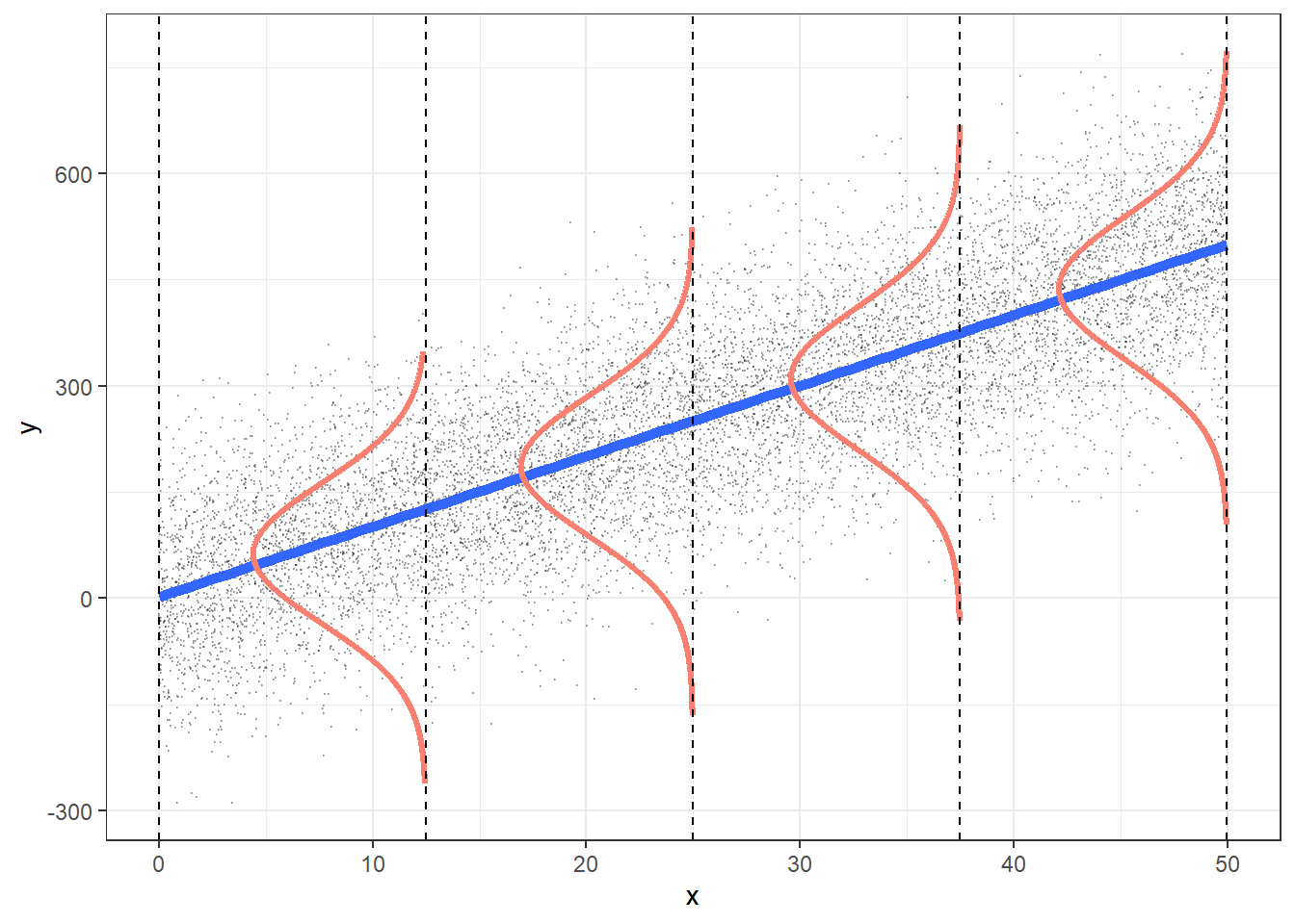
Figure 4.4: Regression and some of its assumptions

Among the assumptions of the linear model are:

linearity of the function
variance of \(y\) remains constant across range of \(x\)
normality of residuals

4.2.4 The linear model

Here’s the canonical form of the linear model.

Consider a model with \(k\) predictors:

\[y = \beta_0 + \beta_1 x_1 + \ldots + \beta_k x_k + \epsilon\]

4.2.5 Algebraic derivation

For the mathematical inclined, check out this derivation of the simple case regression model. Note that the article is written in German, but your browser can effortlessly translate into English. Here’s a similar English article from StackExchange.

4.2.6 The linear model in all its glory

Let’s depict the residuals, s. Figure 4.5.

Figure 4.5: Residuals as deviations from the predicted value

4.2.7 A ladder of common regression formula variants

The following “ladder” shows the logical structure of common linear model in increasing complexity.

Note:

y: the dependent variable
x: a metric independent variable
b: a binary (dichotomic) independent variable
g: a nominal (two or more groups) independent variable
_c: a centered variable

y ~ 1 - the simple grand mean value
y ~ b - difference between two mean values
y ~ g - differences between multiple mean values
y ~ x_c - y as a linear function of x
y ~ x1_c + x2_c - y as a linear function of both x1 and x2
y ~ x_c + g + x_c:g - the interaction (moderator) model
log(y) ~ x1 + x2 - multiplicative association of independent variables
log(p/(1-p)) ~ x - logistic regression

4.3 A simple model: one metric predictor

Note

All the R-code for each chapter can be found as pure, R-only files here. \(\square\)

First, let’s load some data:

data(mtcars)
glimpse(mtcars)  # don't forget to start the "tidyverse package" upfront

Rows: 32
Columns: 11
$ mpg  <dbl> 21.0, 21.0, 22.8, 21.4, 18.7, 18.1, 14.3, 24.4, 22.8, 19.2, 17.8,…
$ cyl  <dbl> 6, 6, 4, 6, 8, 6, 8, 4, 4, 6, 6, 8, 8, 8, 8, 8, 8, 4, 4, 4, 4, 8,…
$ disp <dbl> 160.0, 160.0, 108.0, 258.0, 360.0, 225.0, 360.0, 146.7, 140.8, 16…
$ hp   <dbl> 110, 110, 93, 110, 175, 105, 245, 62, 95, 123, 123, 180, 180, 180…
$ drat <dbl> 3.90, 3.90, 3.85, 3.08, 3.15, 2.76, 3.21, 3.69, 3.92, 3.92, 3.92,…
$ wt   <dbl> 2.620, 2.875, 2.320, 3.215, 3.440, 3.460, 3.570, 3.190, 3.150, 3.…
$ qsec <dbl> 16.46, 17.02, 18.61, 19.44, 17.02, 20.22, 15.84, 20.00, 22.90, 18…
$ vs   <dbl> 0, 0, 1, 1, 0, 1, 0, 1, 1, 1, 1, 0, 0, 0, 0, 0, 0, 1, 1, 1, 1, 0,…
$ am   <dbl> 1, 1, 1, 0, 0, 0, 0, 0, 0, 0, 0, 0, 0, 0, 0, 0, 0, 1, 1, 1, 0, 0,…
$ gear <dbl> 4, 4, 4, 3, 3, 3, 3, 4, 4, 4, 4, 3, 3, 3, 3, 3, 3, 4, 4, 4, 3, 3,…
$ carb <dbl> 4, 4, 1, 1, 2, 1, 4, 2, 2, 4, 4, 3, 3, 3, 4, 4, 4, 1, 2, 1, 1, 2,…

4.3.1 Frequentist

Define and fit the model:

lm1_freq <- lm(mpg ~ hp, data = mtcars)

Get the parameter values:

parameters(lm1_freq)

Parameter	Coefficient	SE	CI	CI_low	CI_high	t	df_error	p
(Intercept)	30.0988605	1.6339210	0.95	26.7619488	33.4357723	18.421246	30	0e+00
hp	-0.0682283	0.0101193	0.95	-0.0888947	-0.0475619	-6.742388	30	2e-07

Plot the model parameters:

plot(parameters(lm1_freq))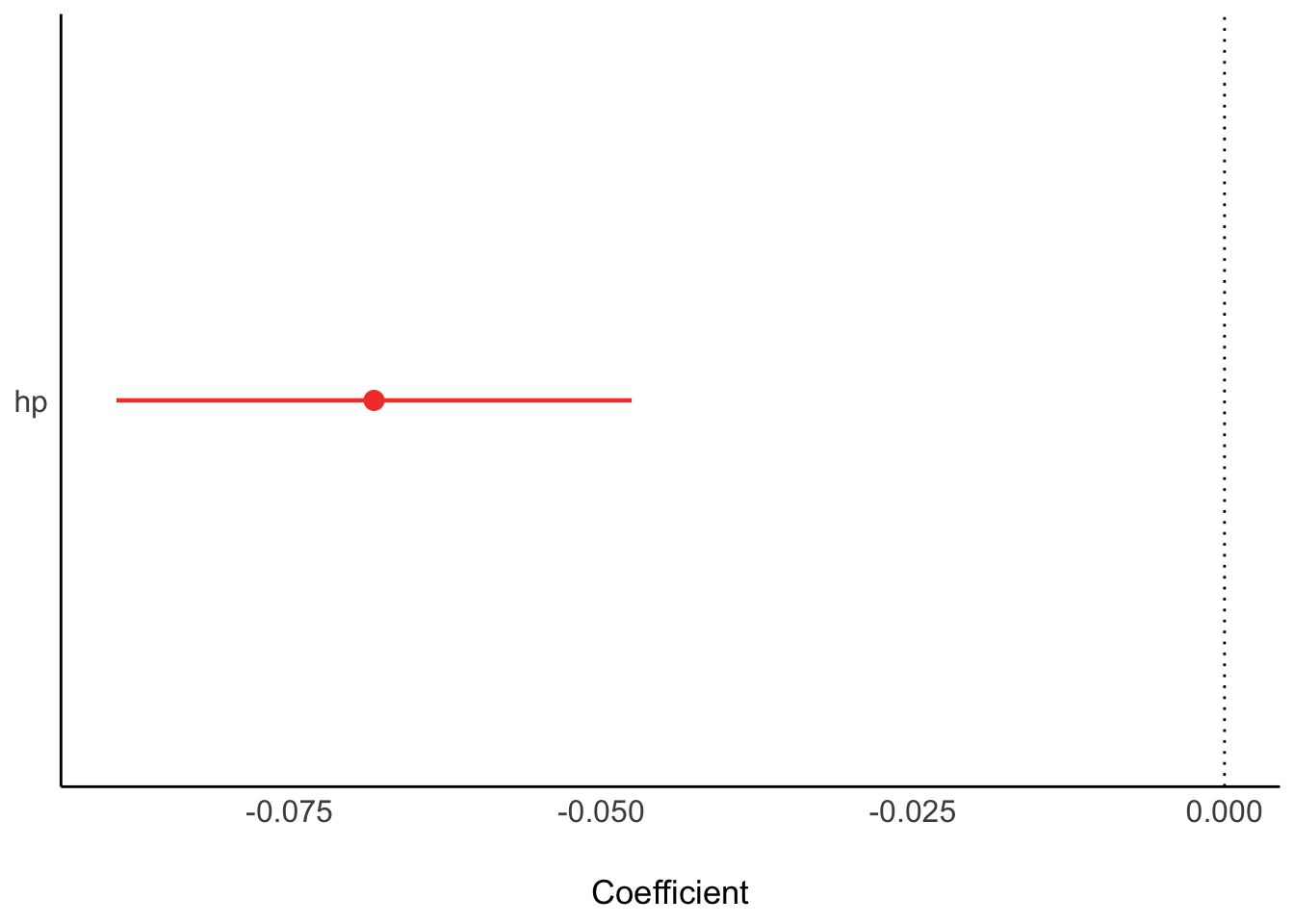

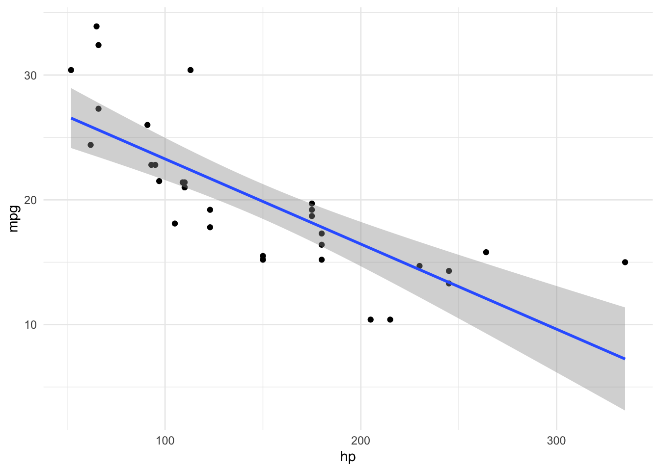
Plot the regression line:

estimate_prediction(lm1_freq, by = "hp") |> 
  plot() +
  geom_point(aes(y = mpg, x = hp), data = mtcars)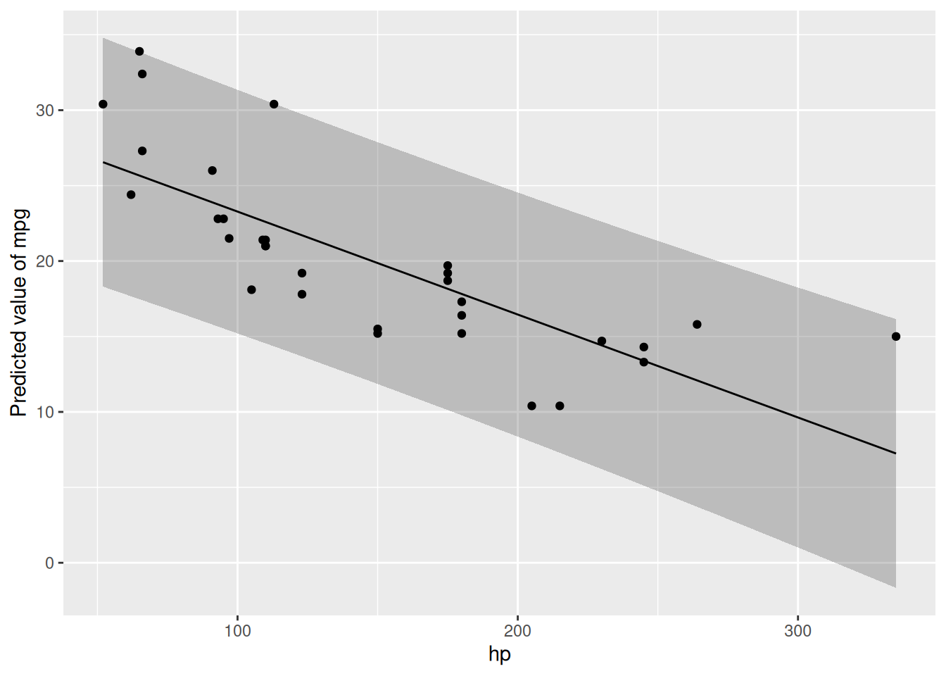

4.3.2 Bayesian

lm1_bayes <- stan_glm(mpg ~ hp, data = mtcars)


SAMPLING FOR MODEL 'continuous' NOW (CHAIN 1).
Chain 1: 
Chain 1: Gradient evaluation took 0.000423 seconds
Chain 1: 1000 transitions using 10 leapfrog steps per transition would take 4.23 seconds.
Chain 1: Adjust your expectations accordingly!
Chain 1: 
Chain 1: 
Chain 1: Iteration:    1 / 2000 [  0%]  (Warmup)
Chain 1: Iteration:  200 / 2000 [ 10%]  (Warmup)
Chain 1: Iteration:  400 / 2000 [ 20%]  (Warmup)
Chain 1: Iteration:  600 / 2000 [ 30%]  (Warmup)
Chain 1: Iteration:  800 / 2000 [ 40%]  (Warmup)
Chain 1: Iteration: 1000 / 2000 [ 50%]  (Warmup)
Chain 1: Iteration: 1001 / 2000 [ 50%]  (Sampling)
Chain 1: Iteration: 1200 / 2000 [ 60%]  (Sampling)
Chain 1: Iteration: 1400 / 2000 [ 70%]  (Sampling)
Chain 1: Iteration: 1600 / 2000 [ 80%]  (Sampling)
Chain 1: Iteration: 1800 / 2000 [ 90%]  (Sampling)
Chain 1: Iteration: 2000 / 2000 [100%]  (Sampling)
Chain 1: 
Chain 1:  Elapsed Time: 0.035 seconds (Warm-up)
Chain 1:                0.033 seconds (Sampling)
Chain 1:                0.068 seconds (Total)
Chain 1: 

SAMPLING FOR MODEL 'continuous' NOW (CHAIN 2).
Chain 2: 
Chain 2: Gradient evaluation took 1.4e-05 seconds
Chain 2: 1000 transitions using 10 leapfrog steps per transition would take 0.14 seconds.
Chain 2: Adjust your expectations accordingly!
Chain 2: 
Chain 2: 
Chain 2: Iteration:    1 / 2000 [  0%]  (Warmup)
Chain 2: Iteration:  200 / 2000 [ 10%]  (Warmup)
Chain 2: Iteration:  400 / 2000 [ 20%]  (Warmup)
Chain 2: Iteration:  600 / 2000 [ 30%]  (Warmup)
Chain 2: Iteration:  800 / 2000 [ 40%]  (Warmup)
Chain 2: Iteration: 1000 / 2000 [ 50%]  (Warmup)
Chain 2: Iteration: 1001 / 2000 [ 50%]  (Sampling)
Chain 2: Iteration: 1200 / 2000 [ 60%]  (Sampling)
Chain 2: Iteration: 1400 / 2000 [ 70%]  (Sampling)
Chain 2: Iteration: 1600 / 2000 [ 80%]  (Sampling)
Chain 2: Iteration: 1800 / 2000 [ 90%]  (Sampling)
Chain 2: Iteration: 2000 / 2000 [100%]  (Sampling)
Chain 2: 
Chain 2:  Elapsed Time: 0.032 seconds (Warm-up)
Chain 2:                0.033 seconds (Sampling)
Chain 2:                0.065 seconds (Total)
Chain 2: 

SAMPLING FOR MODEL 'continuous' NOW (CHAIN 3).
Chain 3: 
Chain 3: Gradient evaluation took 1.6e-05 seconds
Chain 3: 1000 transitions using 10 leapfrog steps per transition would take 0.16 seconds.
Chain 3: Adjust your expectations accordingly!
Chain 3: 
Chain 3: 
Chain 3: Iteration:    1 / 2000 [  0%]  (Warmup)
Chain 3: Iteration:  200 / 2000 [ 10%]  (Warmup)
Chain 3: Iteration:  400 / 2000 [ 20%]  (Warmup)
Chain 3: Iteration:  600 / 2000 [ 30%]  (Warmup)
Chain 3: Iteration:  800 / 2000 [ 40%]  (Warmup)
Chain 3: Iteration: 1000 / 2000 [ 50%]  (Warmup)
Chain 3: Iteration: 1001 / 2000 [ 50%]  (Sampling)
Chain 3: Iteration: 1200 / 2000 [ 60%]  (Sampling)
Chain 3: Iteration: 1400 / 2000 [ 70%]  (Sampling)
Chain 3: Iteration: 1600 / 2000 [ 80%]  (Sampling)
Chain 3: Iteration: 1800 / 2000 [ 90%]  (Sampling)
Chain 3: Iteration: 2000 / 2000 [100%]  (Sampling)
Chain 3: 
Chain 3:  Elapsed Time: 0.056 seconds (Warm-up)
Chain 3:                0.037 seconds (Sampling)
Chain 3:                0.093 seconds (Total)
Chain 3: 

SAMPLING FOR MODEL 'continuous' NOW (CHAIN 4).
Chain 4: 
Chain 4: Gradient evaluation took 1.3e-05 seconds
Chain 4: 1000 transitions using 10 leapfrog steps per transition would take 0.13 seconds.
Chain 4: Adjust your expectations accordingly!
Chain 4: 
Chain 4: 
Chain 4: Iteration:    1 / 2000 [  0%]  (Warmup)
Chain 4: Iteration:  200 / 2000 [ 10%]  (Warmup)
Chain 4: Iteration:  400 / 2000 [ 20%]  (Warmup)
Chain 4: Iteration:  600 / 2000 [ 30%]  (Warmup)
Chain 4: Iteration:  800 / 2000 [ 40%]  (Warmup)
Chain 4: Iteration: 1000 / 2000 [ 50%]  (Warmup)
Chain 4: Iteration: 1001 / 2000 [ 50%]  (Sampling)
Chain 4: Iteration: 1200 / 2000 [ 60%]  (Sampling)
Chain 4: Iteration: 1400 / 2000 [ 70%]  (Sampling)
Chain 4: Iteration: 1600 / 2000 [ 80%]  (Sampling)
Chain 4: Iteration: 1800 / 2000 [ 90%]  (Sampling)
Chain 4: Iteration: 2000 / 2000 [100%]  (Sampling)
Chain 4: 
Chain 4:  Elapsed Time: 0.034 seconds (Warm-up)
Chain 4:                0.037 seconds (Sampling)
Chain 4:                0.071 seconds (Total)
Chain 4:

Actually, we want to suppress some overly verbose output of the sampling, so add the argument refresh = 0:

lm1_bayes <- stan_glm(mpg ~ hp, data = mtcars, refresh = 0)

4.3.3 Model parameters

Get the parameter values:

parameters(lm1_bayes)

Parameter	Median	CI	CI_low	CI_high	pd	Rhat	ESS	Prior_Distribution	Prior_Location	Prior_Scale
(Intercept)	30.1271159	0.95	26.760846	33.3711909	1	1.000212	3514.811	normal	20.09062	15.0673701
hp	-0.0680751	0.95	-0.088685	-0.0472875	1	1.000639	3617.460	normal	0.00000	0.2197599

parameters(lm1_freq)

Parameter	Coefficient	SE	CI	CI_low	CI_high	t	df_error	p
(Intercept)	30.0988605	1.6339210	0.95	26.7619488	33.4357723	18.421246	30	0e+00
hp	-0.0682283	0.0101193	0.95	-0.0888947	-0.0475619	-6.742388	30	2e-07

Plot the model parameters:

plot(parameters(lm1_bayes))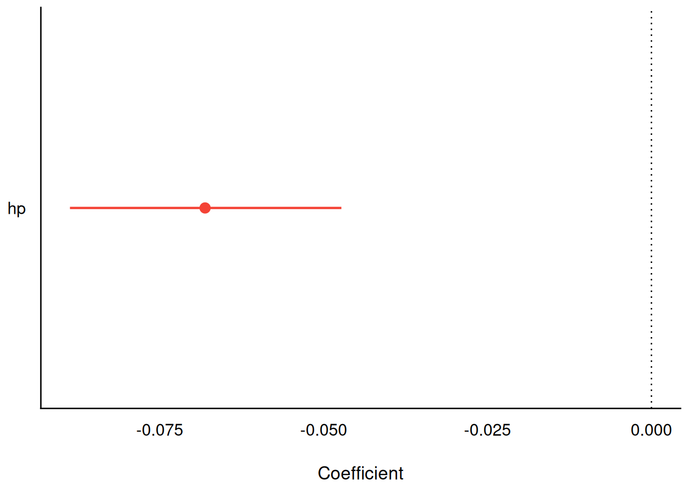

Get some predictions

lm1_pred <- estimate_relation(lm1_freq)
lm1_pred

hp	Predicted	SE	CI_low	CI_high
52.000	26.550990	1.1766139	24.148024	28.95396
83.444	24.405620	0.9358964	22.494265	26.31698
114.889	22.260182	0.7548966	20.718477	23.80189
146.333	20.114812	0.6828911	18.720162	21.50946
177.778	17.969374	0.7518707	16.433849	19.50490
209.222	15.824004	0.9310050	13.922638	17.72537
240.667	13.678565	1.1707869	11.287500	16.06963
272.111	11.533196	1.4412468	8.589777	14.47661
303.556	9.387757	1.7280527	5.858603	12.91691
335.000	7.242387	2.0242544	3.108308	11.37647

More details on the above function can be found on the respective page at the easystats site.

Plot the model (regression line):

plot(lm1_pred) +
  geom_point(aes(y = mpg, x = hp), data = mtcars)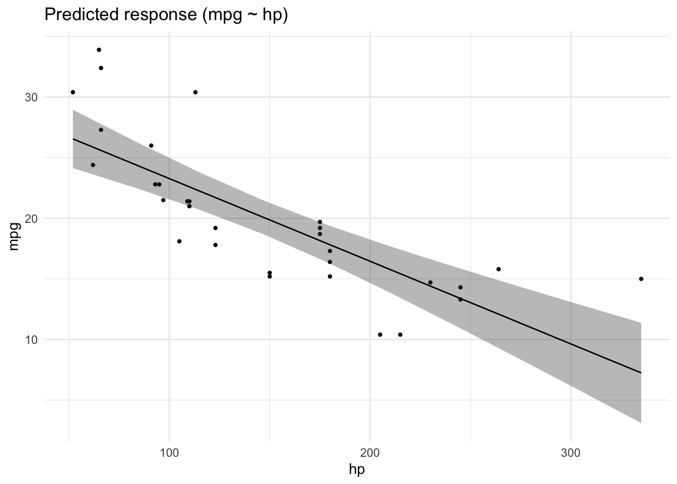

4.3.4 Model performance

r2(lm1_freq)

# R2 for Linear Regression
       R2: 0.602
  adj. R2: 0.589

r2(lm1_bayes)

# Bayesian R2 with Compatibility Interval

  Conditional R2: 0.588 (95% CI [0.373, 0.753])

4.3.5 Model check

Here’s a bunch of typical model checks in the Frequentist sense.

check_model(lm1_freq)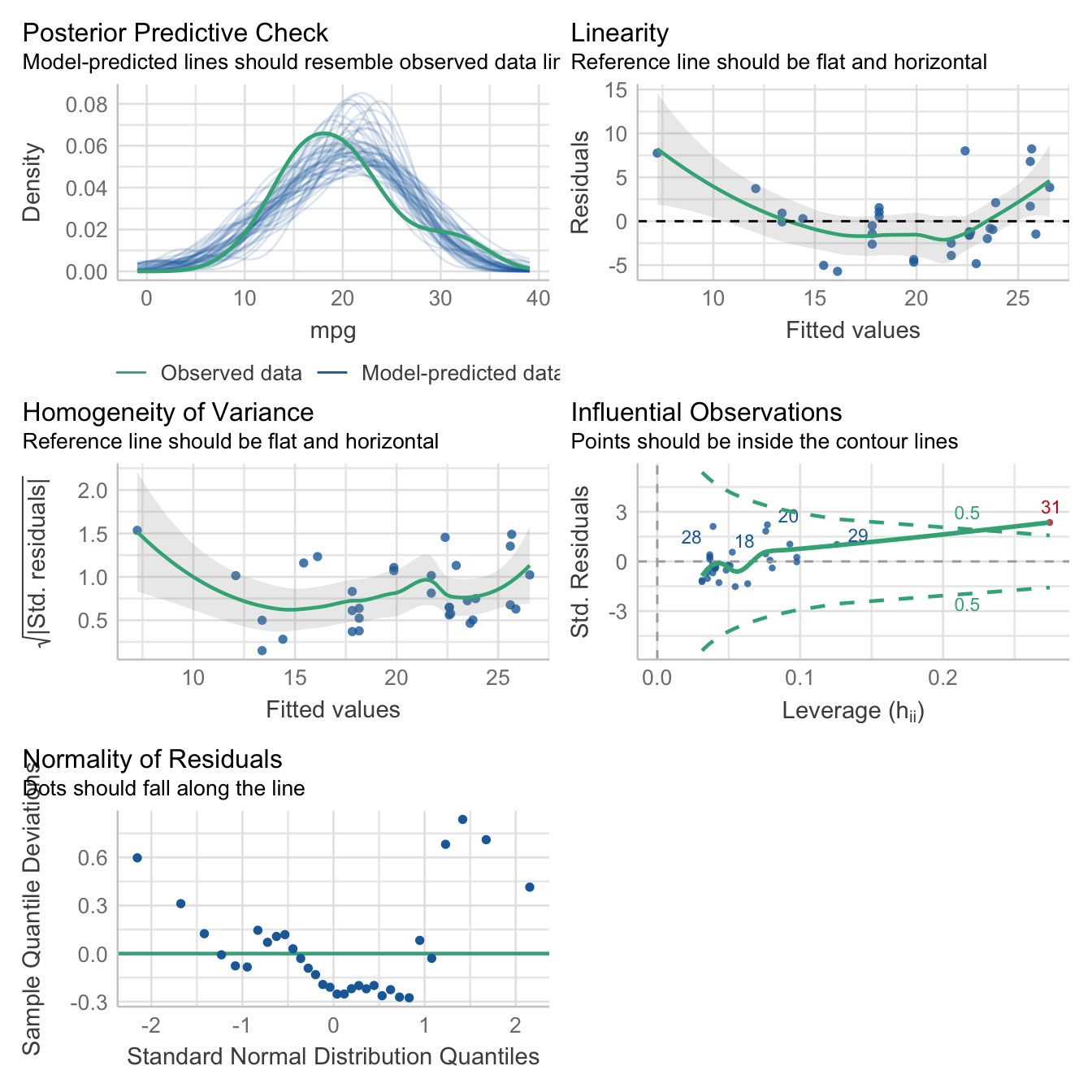

And here are some Bayesian flavored model checks.

check_model(lm1_bayes)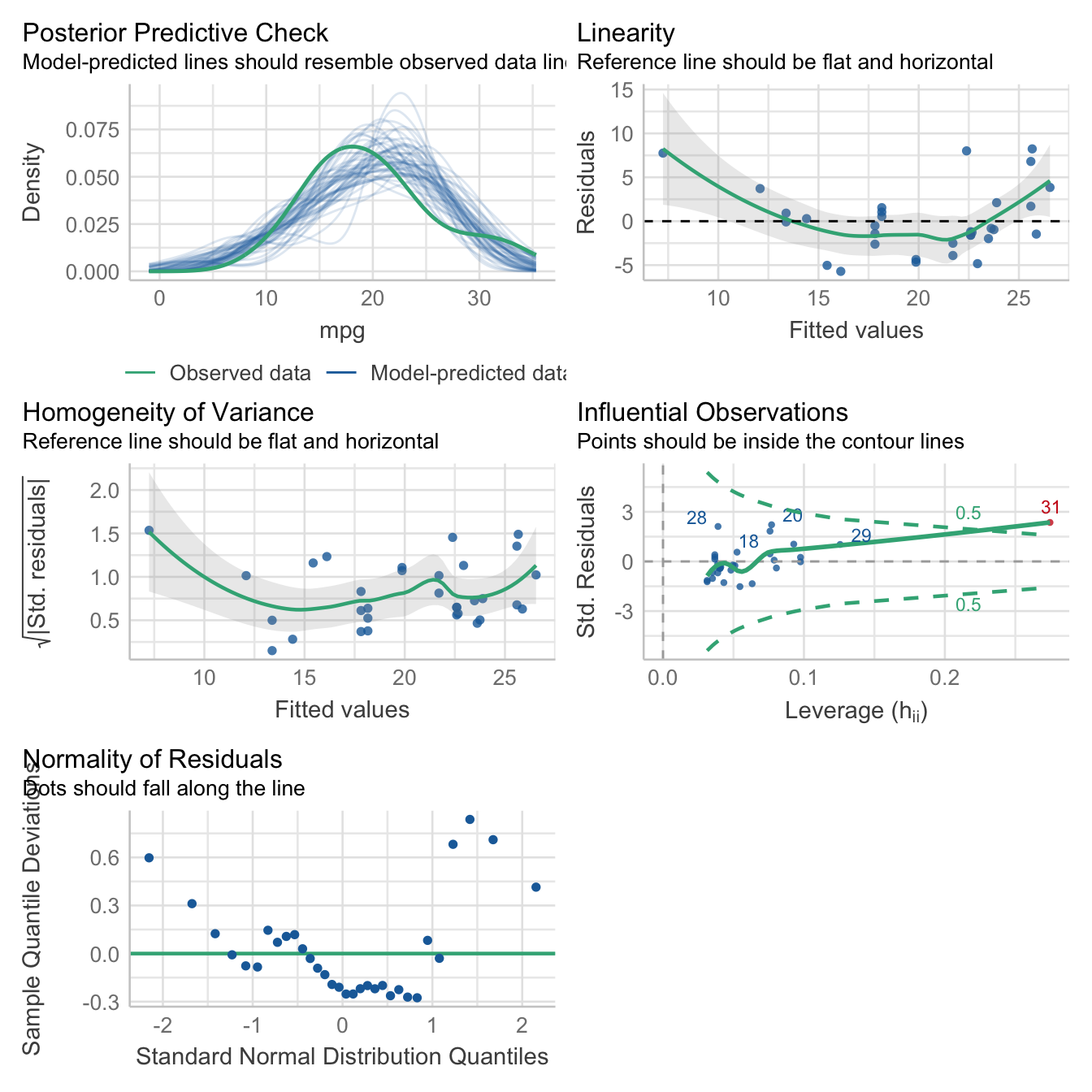

Let’s have a look at the predictions and the residuals:

mtcars <-
  mtcars |> 
  mutate(pred = predict(lm1_bayes),
         resid = resid(lm1_bayes))

gghistogram(mtcars, 
            x = "resid")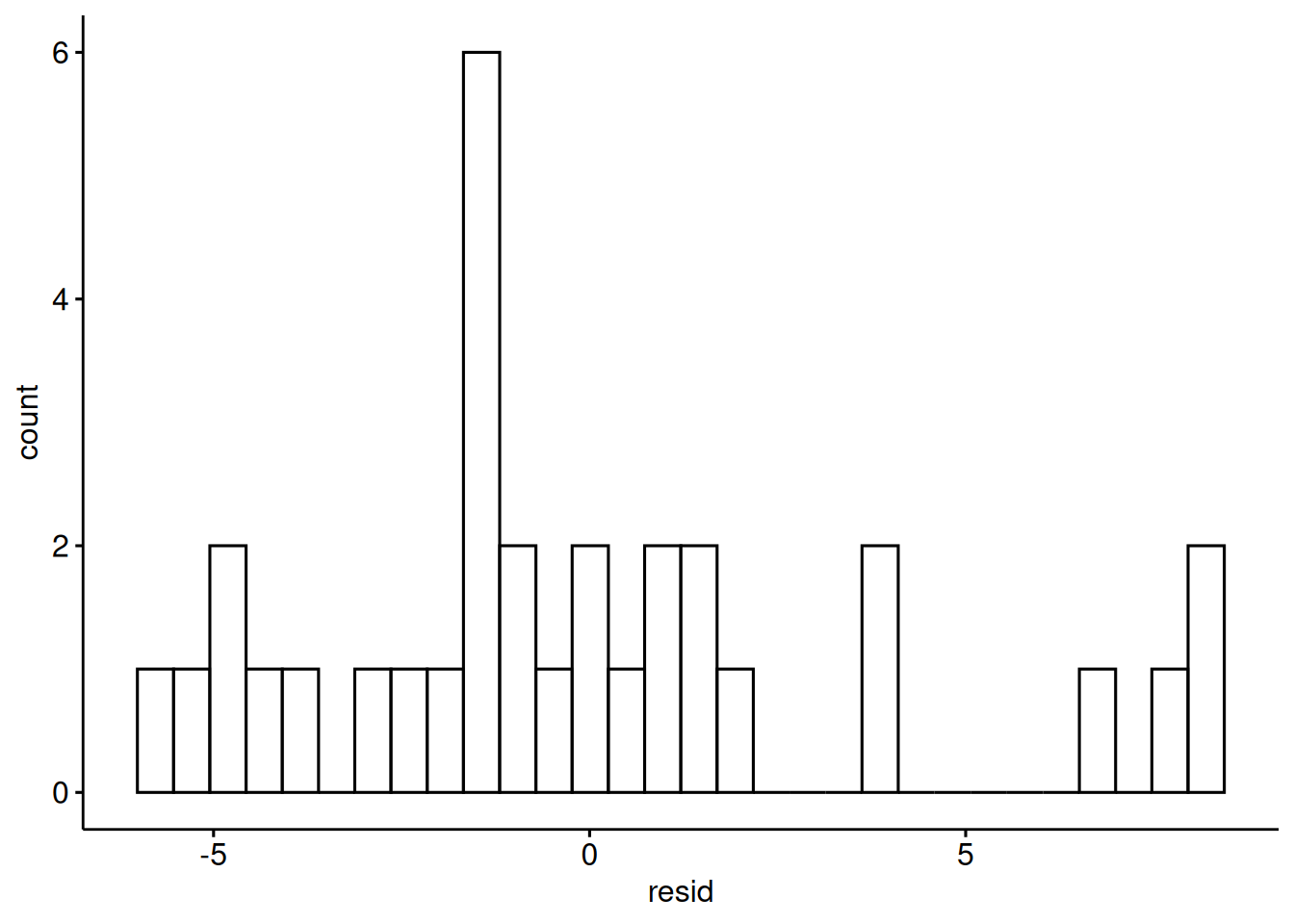

Looks okay.

4.3.6 More of this

More technical details for gauging model performance and model quality, can be found on the site of the R package “performance at the easystats site.

4.3.7 Exercises

See Datenwerk with tag “#regression”.

4.3.8 Lab

Run a simple regression on your own research data. Present the results. Did you encounter any glitches?

4.4 Bayes-members only

Bayes statistics provide a distribution as the result of the analysis, the posterior distribution, which provides us with quite some luxury.

As the posterior distribution manifests itself by a number of samples, we can easily filter and manipulate this sample distribution in order to ask some interesing questions.

See

lm1_bayes_tibble <- as_tibble(lm1_bayes)  # cast as a tibble (table)

head(lm1_bayes_tibble)  # show the first few rows

(Intercept)	hp	sigma
28.84148	-0.0716195	4.224321
32.40379	-0.0773078	3.943005
28.26745	-0.0616808	3.838316
33.07188	-0.0830290	4.403910
30.84380	-0.0711837	3.861623
29.37730	-0.0574441	3.998523

4.4.1 Asking for probabilites

What’s the probability that the effect of hp is negative?

lm1_bayes_tibble %>% 
  count(hp < 0)

hp < 0	n
TRUE	4000

Feel free to ask similar questions!

4.4.2 Asking for quantiles

With a given probability of, say 90%, how large is the effect of hp?

quantile(lm1_bayes_tibble$hp, .9)

        90% 
-0.05458488

What’s the smallest 95% percent interval for the effect of hp?

hdi(lm1_bayes)

Parameter	CI	CI_low	CI_high	Effects	Component
(Intercept)	0.95	26.8240164	33.4168051	fixed	conditional
hp	0.95	-0.0887201	-0.0473449	fixed	conditional

In case you prefer 89% intervals (I do!):

hdi(lm1_bayes, ci = .89)

Parameter	CI	CI_low	CI_high	Effects	Component
(Intercept)	0.89	27.5246307	32.8680028	fixed	conditional
hp	0.89	-0.0849041	-0.0512066	fixed	conditional

4.4.3 Model specification

In Bayes statistics, it is customary to specify the model in something like the following way:

\[\begin{aligned} y_i &\sim N(\mu_i,\sigma)\\ \mu_i &= \beta_0 + \beta_1 x_i\\ \beta_0, \beta_1 &\sim N(0, 1) \\ \sigma &\sim E(1) \end{aligned}\]

In this specification, \(N\) refers to the normal distribution, and \(E\) to the exponential distribution. Furthermore, this model assumes that the \(X\) and \(Y\) are given in standard units.

4.4.4 Prediction interval

A prediction interval answers the following question

How large is the uncertainty in \(y\) associated with a given obersation? What interval of values should I expect for a randomly chosen observation?

For example, what’s the uncertainty attached to the fuel economy of a car with 100 hp?

estimate_prediction(model = lm1_bayes, 
                    data = tibble(hp = 100) )

hp	Predicted	SE	CI_low	CI_high
100	23.26693	4.167489	14.99959	31.42942

4.4.5 … And more

We could even ask intriguing questions such as

Given the model, and given two random observations, one from the experimental group and one from the control group, what is the probability that observation 1 has a higher value in \(Y\) than observation 2 has?

Note that we are not only asking for “typical” observations as predicted by the model but we are also taking into account the uncertainty of the prediction for each group. Hence, this kind of questions is likely to yield more realistic (and less clear-cut) answers than just asking for the typical value. In other words, such analyses draw on the posterior predictive distribution.

4.5 More linear models

4.5.1 Multiple metric predictors

Assume we have a theory that dictates that fuel economy is a (causal) function of horse power and engine displacement.

lm2_freq <- lm(mpg ~ hp + disp, data = mtcars)
parameters(lm2_freq)

Parameter	Coefficient	SE	CI	CI_low	CI_high	t	df_error	p
(Intercept)	30.7359042	1.3315661	0.95	28.0125457	33.4592628	23.082522	29	0.0000000
hp	-0.0248401	0.0133855	0.95	-0.0522165	0.0025363	-1.855746	29	0.0736791
disp	-0.0303463	0.0074049	0.95	-0.0454909	-0.0152016	-4.098159	29	0.0003063

Similarly for Bayes inference:

lm2_bayes <- stan_glm(mpg ~ hp + disp, data = mtcars)

Results

parameters(lm2_bayes)

Parameter	Median	CI	CI_low	CI_high	pd	Rhat	ESS	Prior_Distribution	Prior_Location	Prior_Scale
(Intercept)	30.7414461	0.95	27.9174011	33.5256115	1.00	0.9995722	5030.497	normal	20.09062	15.0673701
hp	-0.0249491	0.95	-0.0521502	0.0023749	0.96	1.0025928	1941.692	normal	0.00000	0.2197599
disp	-0.0300386	0.95	-0.0459895	-0.0154262	1.00	1.0017993	1962.035	normal	0.00000	0.1215712

plot(parameters(lm2_bayes))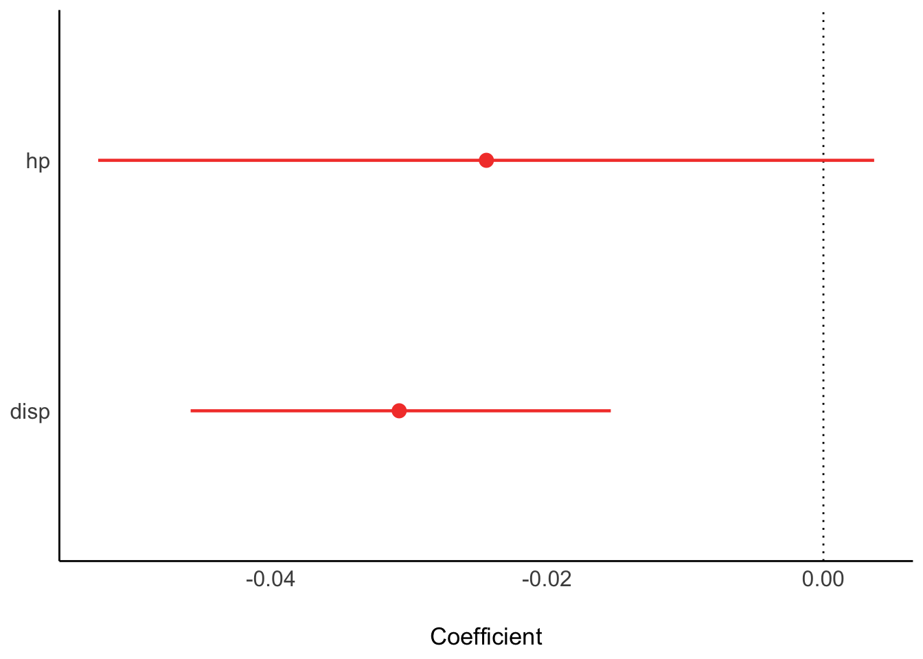

r2(lm2_bayes)

# Bayesian R2 with Compatibility Interval

  Conditional R2: 0.730 (95% CI [0.566, 0.840])

Depending on the value of disp the prediction of mpg from hp will vary:

lm2_pred <- estimate_relation(lm2_freq)
plot(lm2_pred)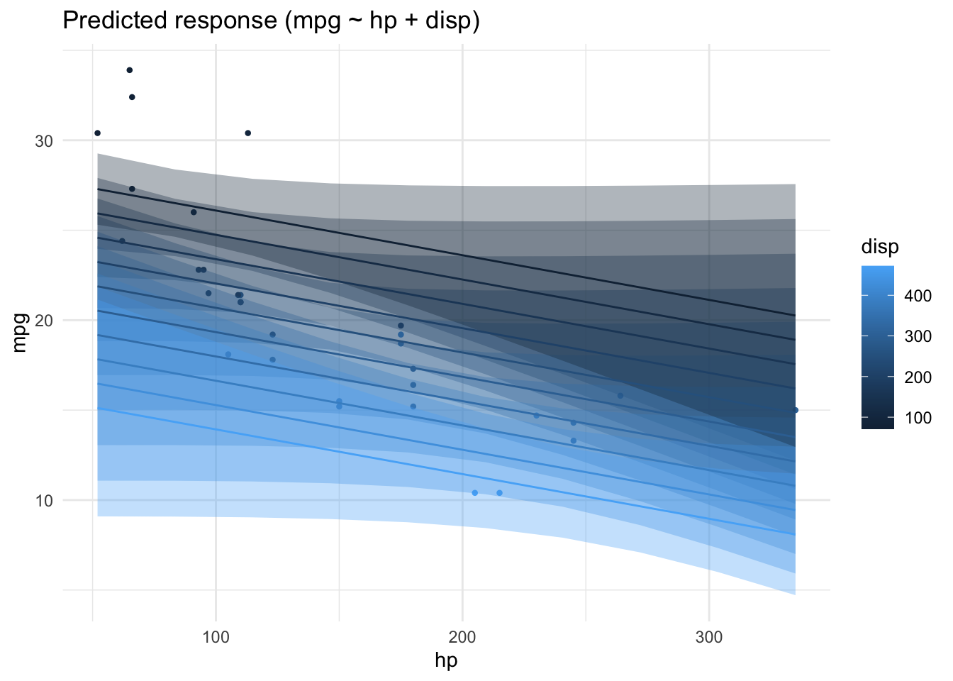

4.5.2 One nominal predictor

lm3a <- lm(mpg ~ am, data = mtcars)
parameters(lm3a)

Parameter	Coefficient	SE	CI	CI_low	CI_high	t	df_error	p
(Intercept)	17.147368	1.124602	0.95	14.85062	19.44411	15.247492	30	0.000000
am	7.244939	1.764422	0.95	3.64151	10.84837	4.106127	30	0.000285

A linear model with one predictor having two values amounts to nothing more than comparing the means of two groups:

ggdotplot(mtcars, x = "am", y = "mpg",
         add = c("mean_se")) +
  labs(caption = "Mean plus/minus SE are shown")

Let’s compute the mean values per group:

mtcars |> 
  group_by(am) |> 
  describe_distribution(select = "mpg")

am	Variable	Mean	SD	IQR	Min	Max	Skewness	Kurtosis	n	n_Missing
0	mpg	17.14737	3.833966	4.50	10.4	24.4	0.0164578	-0.3339353	19	0
1	mpg	24.39231	6.166504	10.05	15.0	33.9	0.0672942	-1.1586082	13	0

However, unfortunately, the plot of the model needs a nominal variable if we are to compare groups. In our case, am is considered a numeric variables, since it consists of numbers only. The plot does not work as expected, malheureusement:

plot(estimate_relation(lm3a))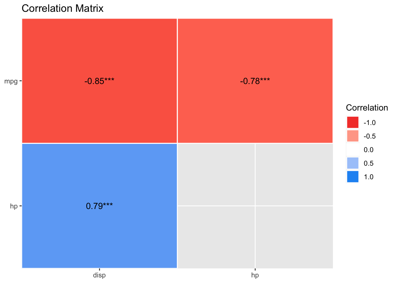

plot(lm3a_means)

Error: Objekt 'lm3a_means' nicht gefunden

We need to transform am to a factor variable. That’s something like a string (text) variable. If we hand over a factor() to the plotting function, everything will run smoothly. Computationwise, no big differences:

mtcars2 <-
  mtcars %>% 
  mutate(am_f = factor(am))

lm3a <- lm(mpg ~ am_f, data = mtcars2)
parameters(lm3a)

Parameter	Coefficient	SE	CI	CI_low	CI_high	t	df_error	p
(Intercept)	17.147368	1.124602	0.95	14.85062	19.44411	15.247492	30	0.000000
am_f1	7.244939	1.764422	0.95	3.64151	10.84837	4.106127	30	0.000285

We can also compute the predicted output values of our model at given input variable values:

lm3a_means <- estimate_means(lm3a, at = "am = c(0, 1)")
lm3a_means

am_f	Mean	SE	CI_low	CI_high	t	df
0	17.14737	1.124602	14.85062	19.44411	15.24749	30
1	24.39231	1.359578	21.61568	27.16894	17.94108	30

If we were not to specify the values of am which we would like to get predictions for, the default of the function would select 10 values, spread across the range of am. For numeric variables, this is usually fine. However, for nominal variables - and am is in fact a nominally scaled variable - we insist that we want predictions for the levels of the variable only, that is for 0 and 1.

lm3a_means <- estimate_means(lm3a)
plot(lm3a_means)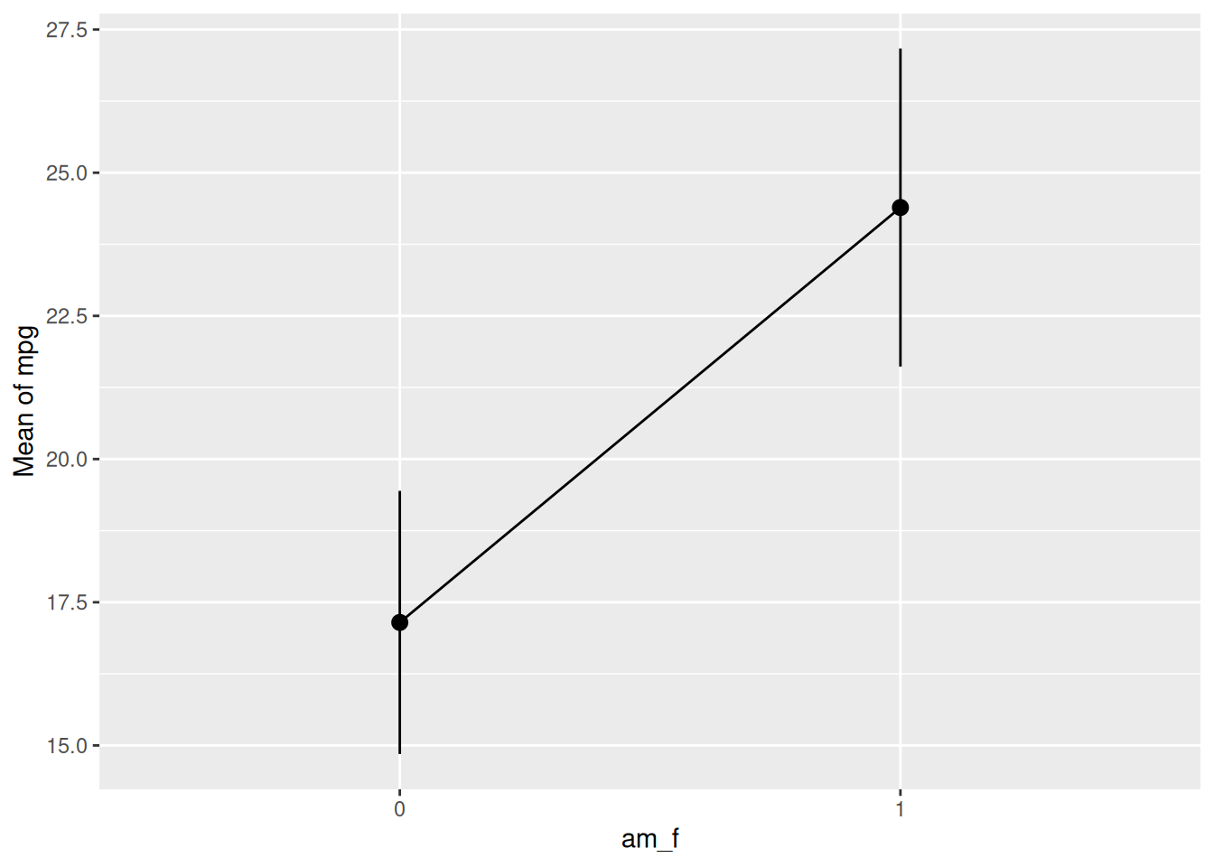

Note that we should have converted am to a factor variable before fitting the model. Otherwise, the plot won’t work.

Here’s a more hand-crafted version of the last plot, see Fig. Figure 4.6.

ggplot(mtcars2) +
  aes(x = am_f, y = mpg) +
  geom_violin() +
  geom_jitter(width = .1, alpha = .5) +
  geom_pointrange(data = lm3a_means,
                  color = "orange",
                  aes(ymin = CI_low, ymax = CI_high, y = Mean)) +
  geom_line(data = lm3a_means, aes(y = Mean, group = 1))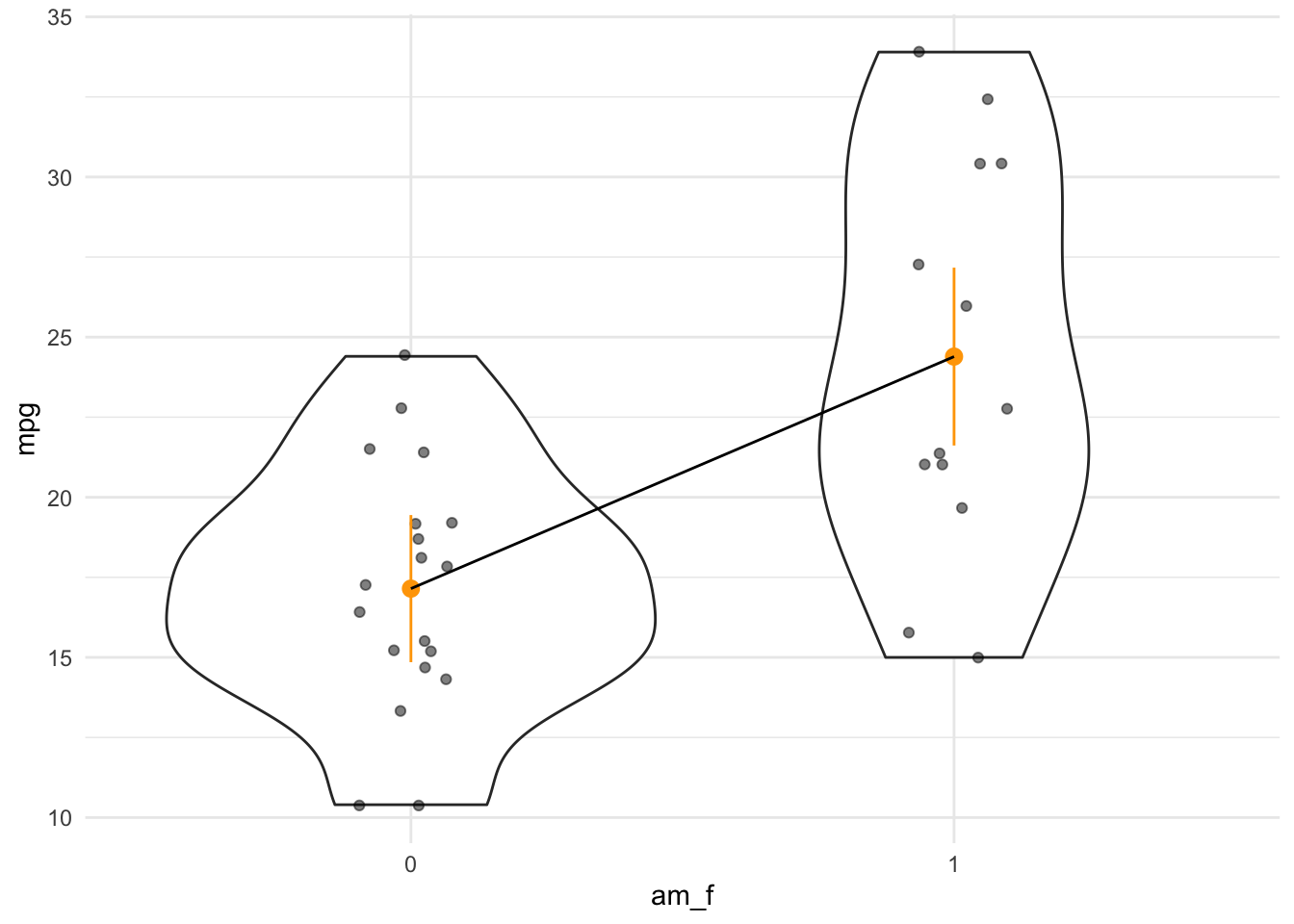

4.5.3 One metric and one nominal predictor

mtcars2 <-
  mtcars %>% 
  mutate(cyl = factor(cyl))

lm4 <- lm(mpg ~ hp + cyl, data = mtcars2)
parameters(lm4)

Parameter	Coefficient	SE	CI	CI_low	CI_high	t	df_error	p
(Intercept)	28.6501182	1.5877870	0.95	25.3976840	31.9025524	18.044056	28	0.0000000
hp	-0.0240388	0.0154079	0.95	-0.0556005	0.0075228	-1.560163	28	0.1299540
cyl6	-5.9676551	1.6392776	0.95	-9.3255631	-2.6097471	-3.640418	28	0.0010921
cyl8	-8.5208508	2.3260749	0.95	-13.2855993	-3.7561022	-3.663188	28	0.0010286

lm4_pred <- estimate_relation(lm4)
plot(lm4_pred)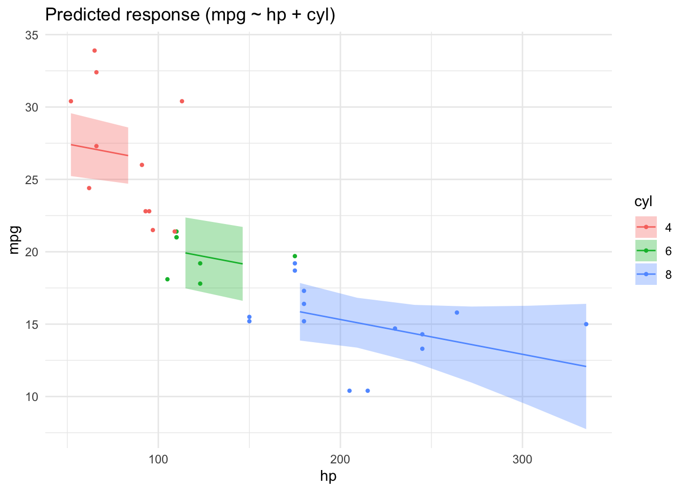

4.5.4 Watch out for Simpson

Beware! Model estimates can swing wildly if you add (or remove) some predictor from your model. See this post for an demonstration.

4.5.5 Quadrat models are also linear

Let’s simulate some data, where \(X\) and \(Y\) are associated in a quadratic manner:

x <- abs(rnorm(n = 100, sd = 3))
e <- rnorm(100)
y <- x^2 + e

d_square <-
  data.frame(
    x = x,
    e = e,
    y = y
  )

Here’s a scatterplot of the data:

ggscatter(d_square,
          x = "x",
          y = "y")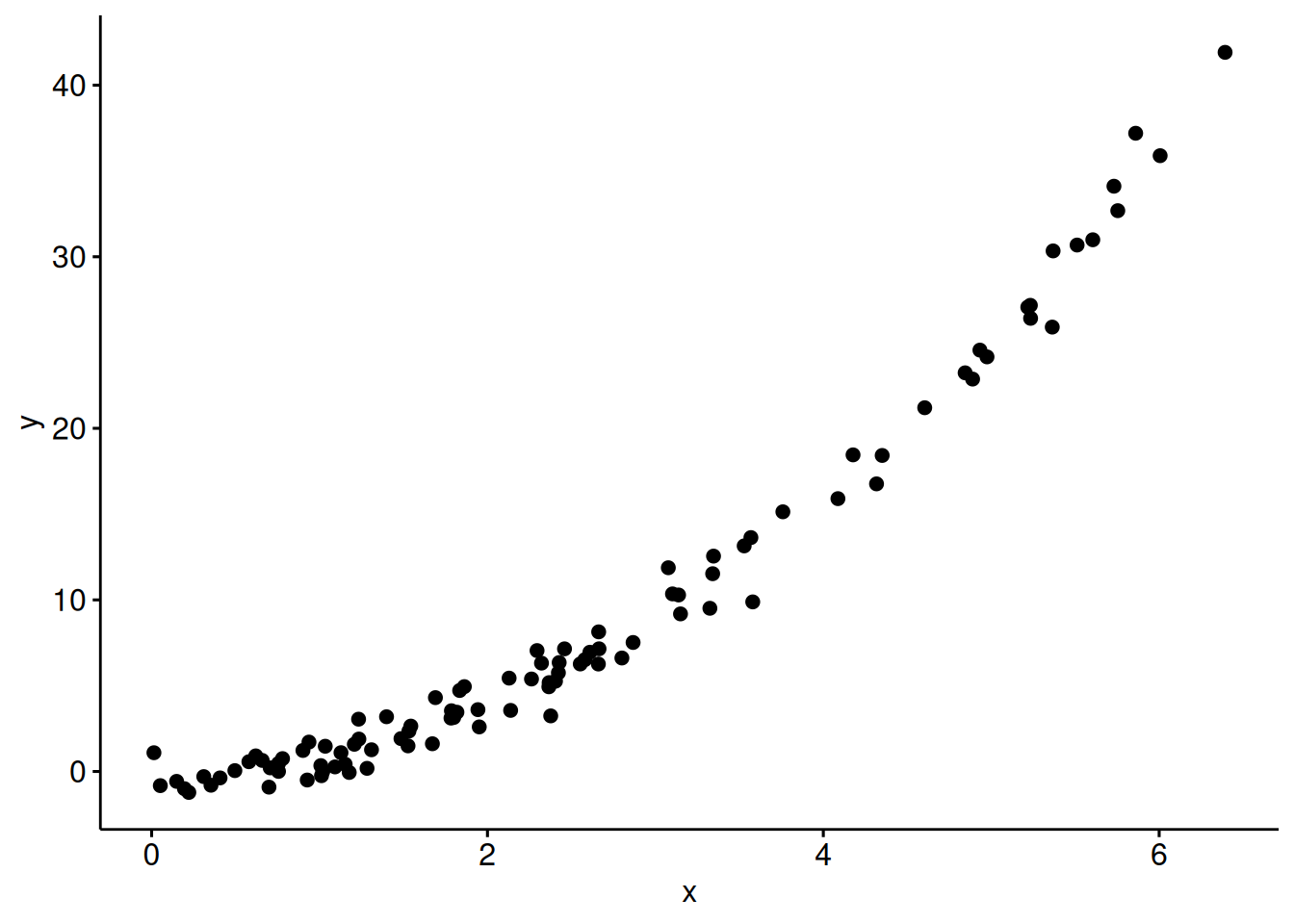

Here’s a “quadratic linear” model:

lm_square <-
  lm(y ~ I(x^2) + x, data = d_square)

Note x^2 in a regression formula is not understood as arithmetic squaring. Hence, we need the I().

parameters(lm_square)

Parameter	Coefficient	SE	CI	CI_low	CI_high	t	df_error	p
(Intercept)	-0.3513295	0.2865703	0.95	-0.9200923	0.2174334	-1.2259798	97	0.2231743
I(x^2)	0.9870886	0.0375881	0.95	0.9124867	1.0616905	26.2606916	97	0.0000000
x	0.1465346	0.2331559	0.95	-0.3162154	0.6092845	0.6284831	97	0.5311646

Here’s our quadratic trend:

estimate_relation(lm_square) |> 
  plot() +
  geom_point(aes(x = x, y = y), data = d_square)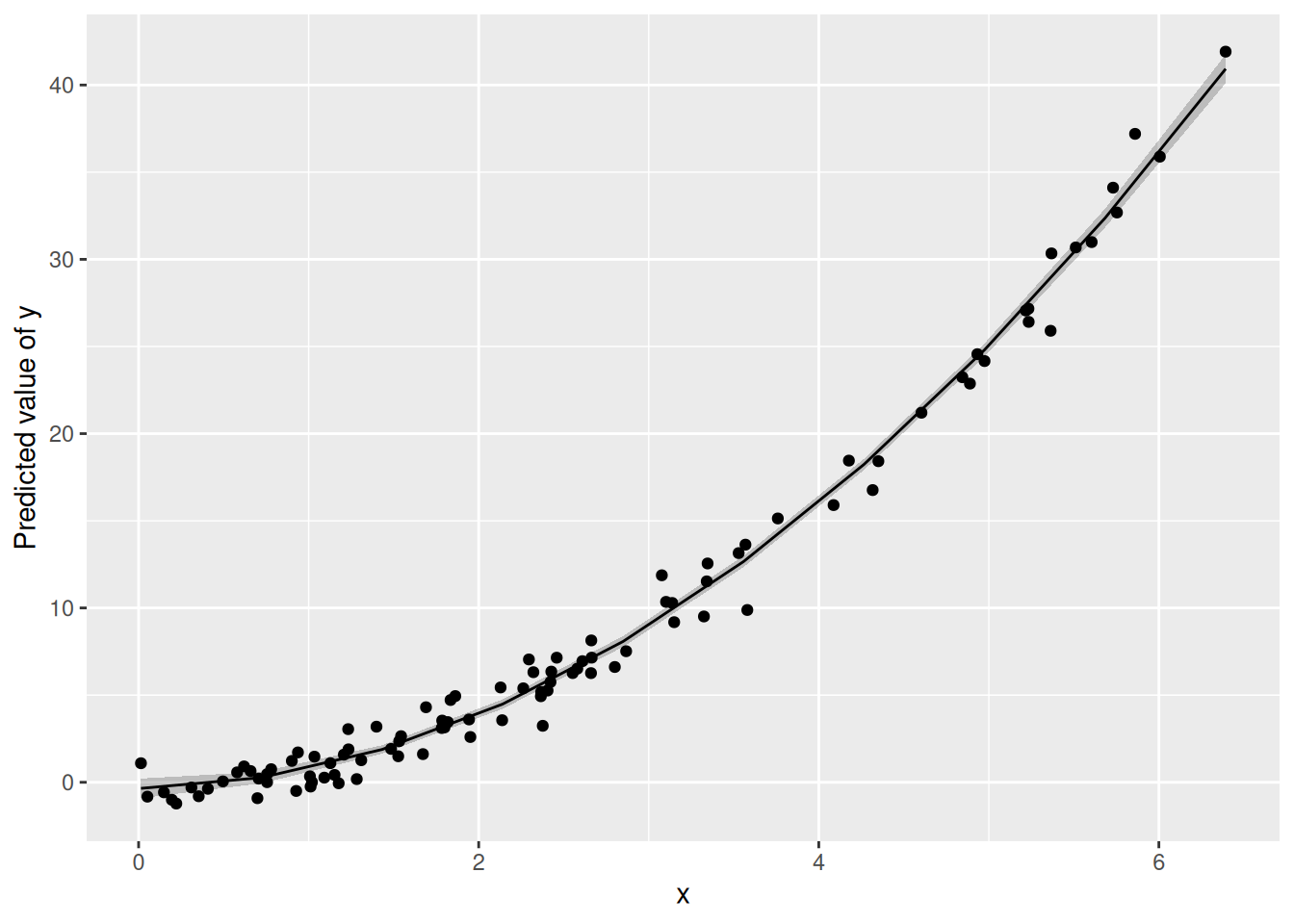

Why is this quadratic model considered linear?

Because \(y\) is a linear function of the betas; the x-es are seen as constants:

\(y = \beta_0 + \beta_1\times x_1 + \beta_2 \times x_2 + \epsilon\),

where \(\x_2\) is the squared value of x.

The same logic applies for other “non-linear” trends such as higher polynomials or exponential trends.

4.6 What about correlation?

Correlation is really a close cousin to regression. In fact, regression with standardized variables amounts to correlation.

Let’s get the correlation matrix of the variables in involved in lm4.

lm4_corr <- 
  mtcars %>% 
  select(mpg, hp, disp) %>% 
  correlation()

lm4_corr

Parameter1	Parameter2	r	CI	CI_low	CI_high	t	df_error	p	Method	n_Obs
mpg	hp	-0.7761684	0.95	-0.8852686	-0.5860994	-6.742388	30	2e-07	Pearson correlation	32
mpg	disp	-0.8475514	0.95	-0.9233594	-0.7081376	-8.747151	30	0e+00	Pearson correlation	32
hp	disp	0.7909486	0.95	0.6106794	0.8932775	7.080122	30	1e-07	Pearson correlation	32

plot(summary(lm4_corr))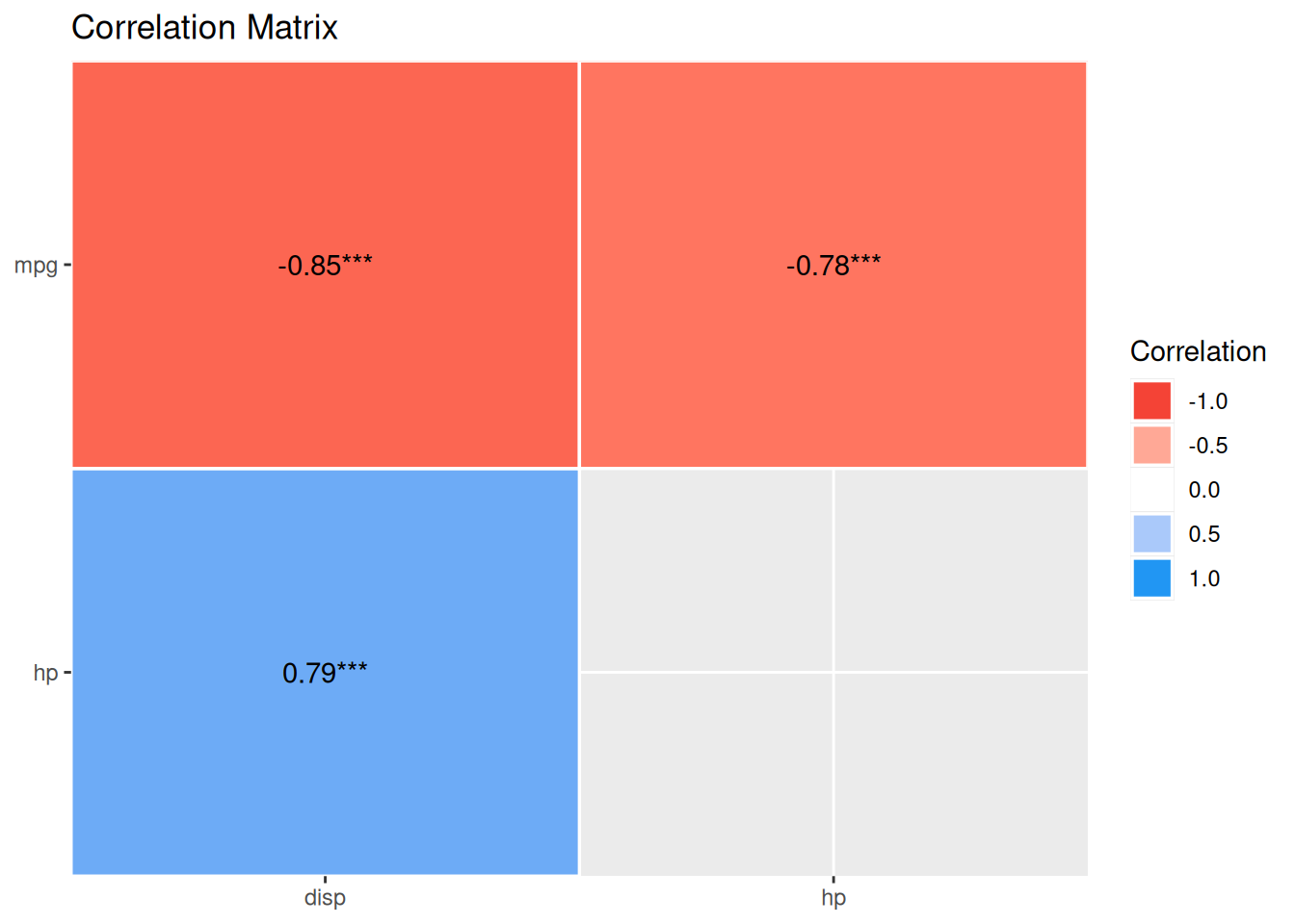

Again, here’s the scatter plot (for mpg as a function of disp):

ggscatter(mtcars,
          x = "disp",
          y = "mpg",
          add = "reg.line")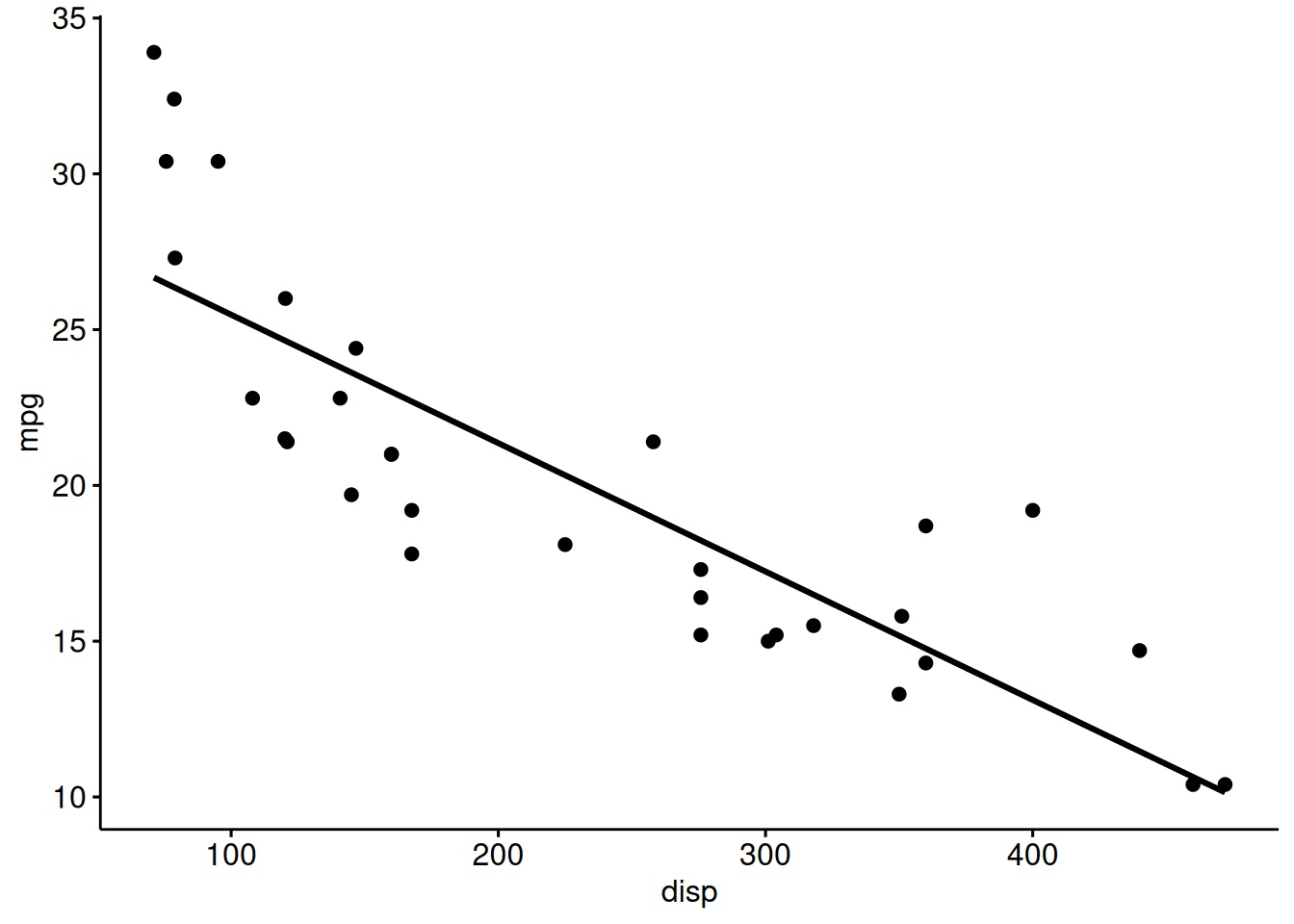

4.7 Exercises

🧑‍🎓 I want more!

👨‍🏫 Checkout all exercises tagged with “regression” on datenwerk. Pro-Tipp: Use the translation function of your browers to translate the webpage into your favorite language.

4.8 Case study

Prices of Boston houses, first part
Modeling movie succes, first part

4.9 Lab

Get your own data, and build a simple model reflecting your research hypothesis. If you are lacking data (or hypothesis) get something close to it.

4.10 Going further

Check-out this chapter of my intro stats book to get an overview on statistical modeling using basic regression technieques. Please use your browser’s translation feature to render the webpages into your favorite language.

An accessible treatment of regression is provided by Ismay & Kim (2020).

Roback & Legler (2021) provide a more than introductory account of regression while being accessible. A recent but already classic book (if this is possible) is the book by Gelman et al. (2021). You may also benefit from Poldrack (2022) (open access).

For a gentle introduction to the basics of modelling, see ModernDive Chap. 5.0 (Ismay & Kim, 2020), and get the R code here. For slightly more advanced topics on linear regression such as multiple regression and interaction, see ModernDive Chap. 6, and get the R code here.

4.11 Debrief

Science!